Representing results on one-dimensional cuts

In order to get a more detailed impression of the quality of a solution, one can show graphs of the function $u(x,y;\varepsilon )$ in the following one-dimensional subsets of $\Omega = \mathbb{R}^2 \setminus \{ (x,y) \vert x^2+y^2 <1 \}$. The following choices seem most relevant:

1. Along fixed vertical cuts
   
   $$\left\{ (x,y)\in \Omega ~\vert~ x=c,~ 0 \le y \le 4 \right\}, \qquad c= -1,0,1,2,4,$$
   
   
   to get an impression of the global behaviour.
2. Along fixed horizontal cuts
   
   $$\left\{ (x,y)\in \Omega ~\vert~ -2 \le x \le 8,~ y = c \right\}, \qquad c= 0,1,$$
   
   
   to get an impression of the global behaviour.
3. Along $\varepsilon$-dependent radial cuts
   
   $$\left\{ (x,y)\in \Omega ~\vert~ x^2 + y^2 = (1 + c ~\varepsilon ^k)^2 \right\}, \qquad~ c= 1; ~~ k= 1, \frac 2 3, \frac 1 2,$$
   
   
   to get an impression of the boundary layer behaviour.
4. Along $\varepsilon$-dependent horizontal cuts
   
   $$\left\{ (x,y)\in \Omega ~\vert~ -2 \le x \le 8,~ y = 1 + c ~\varepsilon ^k \right\}, \qquad c= -1,+1;~~ k= \frac 1 2,$$
   
   
   to get an impression of the interior layer behaviour.

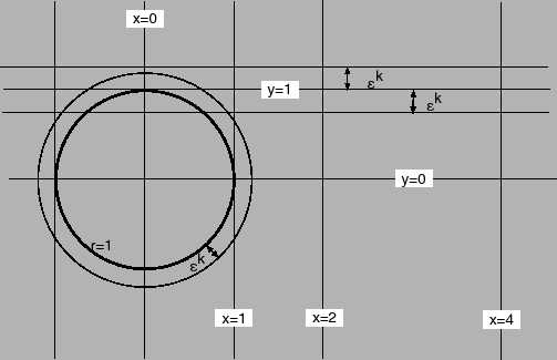
Figure 8: The location of the cuts in the $(x,y)$-plane.

Horizontal cuts along $y=0,1-\varepsilon ^{1/2},1,1+\varepsilon ^{1/2}$, vertical cuts at $x=-1,0,1,2,4$ and radial cuts at $r=1+\varepsilon ^k$, $k= 1, 2/3, 1/3$.

As an example, in the Figures 9, 10 11 and 12 we show results for these cuts for the case $\varepsilon =0.04$.

Figure 9: The solution $u(x,y;\varepsilon )$ along vertical cuts in the $(x,y)$-plane.

$x=-1,0,1,2,4,8,16$;         $-5<y<+5$.

Figure 10: The solution $u(x,y;\varepsilon )$ along radial cuts in the $(x,y)$-plane.

$r=1+\varepsilon ^k$, $k=1,\frac 2 3, \frac 1 2,\frac 1 3$;          $-\pi<\theta<\pi$.

Figure 11: The solution $u(x,y;\varepsilon )$ along horizontal cuts $y=0,1-\varepsilon ^{1/2},1,1+\varepsilon ^{1/2}$ in the $(x,y)$-plane.

$-2<x<4$.

Figure 12: The solution $u(x,y;\varepsilon )$ along horizontal cuts $y=0,1-\varepsilon ^{1/2},1,1+\varepsilon ^{1/2}$ in the $(x,y)$-plane.

$0<x<24$;